Running gSolve for network adjustment on relative gravity readings

Running gSolve for network adjustment on relative gravity readings#

Tip

Example script to process the Okataina data in the examples folder.

import pathlib

try:
    import contextily as cx
except ImportError:
    has_contextily = False
else:
    has_contextily = True

from gsolve import (
    GravityAnomalies,
    GravityCorrectionParameters,
    GravityObservations,
    GravitySites,
    GravitySurvey,
    LaCosteRombergDialConverter,
    ReferenceGravity,
)
from gsolve.tide.earth_tide import LongmanTidalCorrection, EternaPredictTidalCorrection
from gsolve.reports import GSolveReport

Here we assume the data are in an excel spreadsheet (xlsx) with a “Survey Data” and “locations” tab

You can also supply individual csv files for GravitySites and GravityObservations using .from_csv

data_path = pathlib.Path(__file__).parent.parent

obs_path = data_path / "surveys" / "Okataina"

survey_file = obs_path / "Okataina_2020_all_4_gsolve.xlsx"

ref_site_file = data_path / "absolute_gravity" / "base_stations.csv"

corr_table_file = data_path / "correction_tables" / "G106.csv"

The calibration factor for your meter (determined in calibration survey). Previously referred to as the “beta factor” in older gSolve versions.

In previous gui-based gSolve versions the calibration factor (then called beta_factor) was output as a correction to a unit factor of 1 i.e. a beta_factor was a small number close to 0.

To convert your old beta_factor to a calibration factor use calibration_factor = 1 - beta_factor

Tip

If you calculated the calibration factor using gSolve version 5 then just use the calibration factor as is.

Note the calibration factor is used as gcorr = reading * calibration_factor

calibration_factor = 1- -0.0019

Read in the gravity survey data#

Here we create both observation and sites objects. Observations contain the gravity data while sites contain the GNSS location data of each station. Note we have the date time information split into separate “day”, “month”, “year”, “hour”, “minute” columns hence we use parse_split_datetime=True

obs = GravityObservations.from_excel(survey_file, sheet_name="Survey Data", parse_split_datetime=True)

Read in site location information#

sites = GravitySites.from_excel(survey_file, sheet_name="Locations")

Read in list reference (i.e. absolute) stations#

To process the data from relative to absolute we require a list of absolute “reference” stations that the relative survey has occupied.

ref_sites = ReferenceGravity.from_csv(ref_site_file)

set which reference stations are used in this survey (must be in sites)

_ = sites.set_reference_gravity(ref_sites)

Process the observed data#

As this is a manually read G meter we need to convert dial values to mgal via a conversion table. First read in the conversion table

g106converter = LaCosteRombergDialConverter.from_csv(corr_table_file)

apply dial conversion to convert values to mGal.

obs.apply_dial_to_mgal(g106converter)

set the calibration factor

obs.set_calibration_factor(calibration_factor)

Calculate the earth tide correction#

This requires location information from the sites object. There is the option of using the Longman formula or ETERNA Predict with a choice of tidal potential models. Refer to pygtide documentation for other options.

longman = LongmanTidalCorrection(amp_factor=1.2)
obs.apply_earth_tide_correction(sites, tide_corrector = longman)

Another option is to use pygtide for corrections which uses the more accurate ETERNA tidal model.

eterna = EternaPredictTidalCorrection(tidalpoten=8)
obs.apply_earth_tide_correction(sites, tide_corrector = eterna)

Other tidal parameters for Eterna can be set through set_tidal_params once the tide correction object is initialised. e.g. eterna.set_tidal_params([0, 100, 1.15, 0])

Calculate earth tide corrected gravity#

obs.calculate_tide_corrected_gravity()

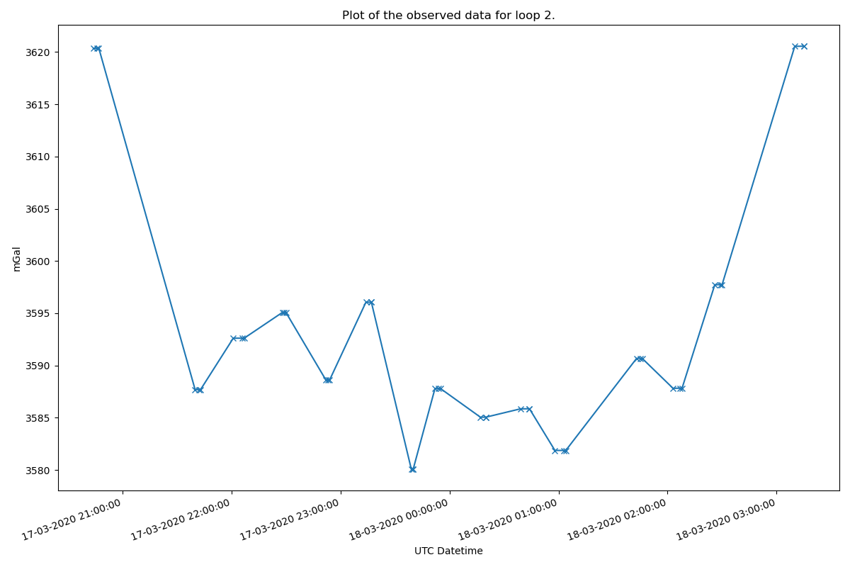
Plot the observed data#

Plot the observed data for each loop to check for input errors. Here we plot for loop #2

obs.plot_observed_data(2, "datetime", "meter_reading_mgal")

observed data

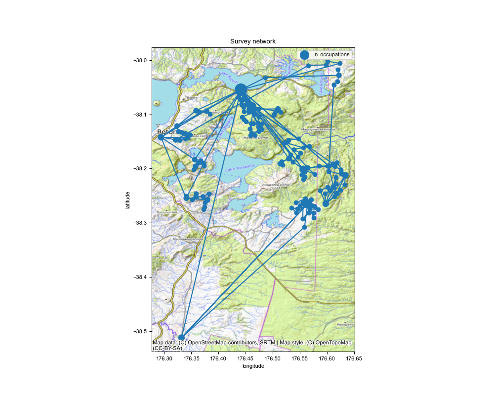
Plot a network map#

Make a map of the network of sites. Dots are scaled by the number of occupations.

fig, ax = obs.plot_network_map(
    sites,
    savefilename=str(obs_path) + "/ Okataina_network_map.png",
    figsize=(10, 8),
    marker_scale_factor=25,
)

# add a basemap (optional)
if has_contextily:
    cx.add_basemap(ax, source=cx.providers.OpenTopoMap, crs="EPSG:4326")
    fig.savefig(str(obs_path) + "/ Okataina_network_map.png")

network map

Create a survey object using observations and site objects#

survey = GravitySurvey(obs, sites)

Run the network adjustment#

Here we use solve method “2”, see gSolve algorithms documentation. We process each loop individually and apply a 99 percentile cutoff filter to the residuals. As this is not a calibration survey we do not need to calculate the calibration factor

results = survey.solve_lstsq(method=2, use_loops=True, calculate_calibration=False, percentile_clipping=95)

Tip

results.site_solution contains the adjusted gravity per station

print(results.site_solution)

Tip

results.obs_solution contains the residuals for each reading.

print(results.obs_solution)

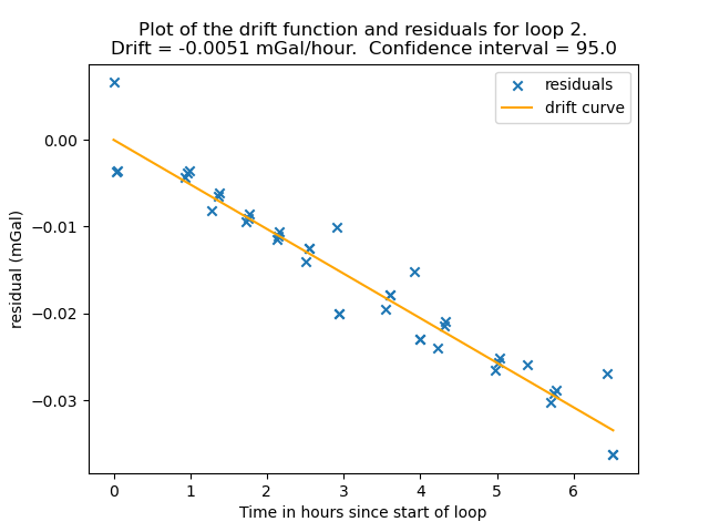
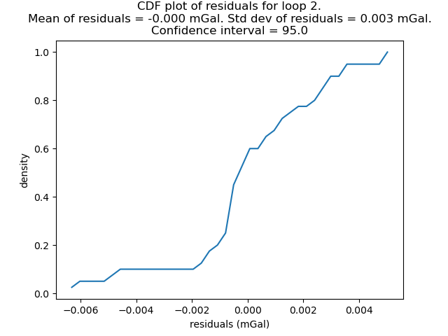
Plot drift and residual curves#

Note: you can use loop=”all” to plot the residual_cdf of all loops together.

results.plot_residual_drift(loop=2, filename=str(obs_path) + "/ Okataina_residual_drift.png")
results.plot_residual_cdf(loop=2, filename=str(obs_path) + "/ Okataina_residual_cdf.png")

residual_drift residual_cdf

Save output files#

as individual csv files

results.site_solution.to_csv(obs_path / "Okataina_site_solution.csv")
results.obs_solution.to_csv(obs_path / "Okataina_observations_solution.csv")

Calculate Corrections and Anomalies#

If you want to carry on and calculate corrections and anomalies.

Define parameters for calculating gravity corections and anomalies.

correction_params = GravityCorrectionParameters(
    ellipsoid="GRS80",
    density_crust=2670.0,
    density_water=1030.0,
    spherical_cap_radius=166735.0,
    use_curvature_corrected=True,
    use_atmospheric_correction=True,
)

use_curvature_corrected applies the Bullard “B” curvature correction for the Bouguer slab. use_atmospheric_correction applies the atmospheric correction for the air mass above the station.

calculate anomalies#

Anomalies are calculated using normal_gravity_at_ellipsoid.

anomalies = GravityAnomalies(
    absolute_gravity=results,
    sites=survey.sites,
    corrections_parameters=correction_params,
    terrain_corrections=None,
)

anomalies.data

Final report#

report = GSolveReport(
    observations=obs,
    results=results,
    sites=survey,
    anomalies=anomalies,
)
report.to_excel(obs_path / "okataina_survey_results.xlsx", if_workbook_exists="replace")